
This is going to be one of the most abstract and technical posts yet; it’s inessential for reading this blog, but I wanted to include it because I would like to cultivate as many different possible viewpoints of scheme theory from the very start. There will be one more post running in this vein and then we will go back to doing actual geometry. However, this post will provide some more structure to the “functor of points” approach we have seen.
Essentially, when learning about the functor of points we saw that every scheme can be viewed as a set-valued presheaf on the opposite of the category of rings (i.e. just a functor from rings to sets, but this is a better viewpoint). But in fact this does not characterise schemes – not every presheaf on the opposite category of rings is the functor of points of a scheme (i.e. not every presheaf on the category of rings is representable). So in order to characterise schemes in this way we will need to find some further structure present. It turns out that with a suitable definition of a “topology” on the (opposite) category of rings – turning this category into something like a space – we will see that schemes are actually the sheaves on this category, which obey the “identity” and “glueing” axioms we looked at in one of the very first posts on this blog.
This post will consist of establishing the vocabulary of these so-called “Grothendieck (pre)topologies” on categories, and we will use these to define sheaves on categories in two ways. In an upcoming post we will use this to see the applicability to schemes, but this is going to be a purely category-theoretic post (and mostly taken from Johnstone’s lovely book Topos Theory). Feel free to skip!
Pretopologies
Let 


into 
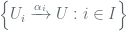
- For every
;
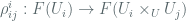
- If
is a morphism in
then
;
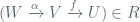
- If
is an element of
is an element of
for each
then the composition
is an element of
Morally, these should be interpreted as follows: if 


As a concrete example, let 

Grothendieck pretopologies already give us enough “local” information in our categories to define a suitable notion of a sheaf on the category. Recall we could define a presheaf on any category as simply a contravariant functor, but in order to define a sheaf we needed to be able to talk about covers, and this is exactly what a pretopology lets us do. With this in mind we say that a presheaf 

is an equaliser. Here the first map is the universal map into the product induced by the restrictions 


be the canonical projections. For each 
Therefore the compositions 


We will use this definition of a sheaf sometimes because it is more closely related to what we have already seen. However it is a slightly vague definition; to see what I mean, suppose that 


This is a far-reaching quasi-generalisation of the fact that two different metrics on a space can induce exactly the same topology (the metrics then being called equivalent) and therefore the sheaves on these spaces (in the usual sense we defined here) will be exactly the same. Given that sheaves are more of a “topological” object and not a “metric” object, it might make sense to get to the root of this and define actual “topologies” on our categories rather than “metrics” (bear in mind this is a very loose analogy!). So we might want to consider covering families which are somehow “maximal”, and this is what the notion of a “sieve” encapsulates. Following this, we can also dispense with the assumption that our category
Topologies
Let 

for every morphism 
Definition: Let 

- The maximal sieve
is an element of
- If
and
is an element of
;
- If
we have
then
.
A category equipped with a (Grothendieck) topology is called a site. This definition implies some important things:
Let 


Note that every Grothendieck pretopology 

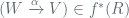
The real benefit of using sieves instead of covering families is that we can drop the assumption about the base category having pullbacks. The reason is that we can always pull a sieve back along a morphism even if we cannot do this for the individual morphisms in the sieve. To see why this works, let

be the representable presheaf on

be the presheaf 


![[\mathcal{C}^\text{op}, \text{Set}]](https://s0.wp.com/latex.php?latex=%5B%5Cmathcal%7BC%7D%5E%5Ctext%7Bop%7D%2C+%5Ctext%7BSet%7D%5D&bg=ffffff&fg=516064&s=0&c=20201002)


Sheaves on a site
A sheaf 

in
Ouch! How abstract can you get???
But there’s a nice way to decode this to see it really isn’t too different to what we already have. Recall that by the Yoneda Lemma, natural transformations 


If 


for each 


Therefore a morphism 


Here are some final notes for this post:
- In the last paragraph we saw how unique “sections”
(corresponding to the inclusion of an open subset), this time there may be many different ways to “restrict a section”; in fact we can do this along each of the different morphisms
- Sometimes it is more useful to work with a topology and other times a pretopology may be better suited. I get the feeling from reading the experts that pretopologies may be more suitable for actually computing things, whereas topologies and sites are more elegant, but really I’m not sure. I’m only beginning to get my head around these things.
Finally, in one of the next few posts I will attempt to use these gadgets to show how every scheme, as we’ve defined them, can also be defined as a sheaf on the Zariski site.

Just found your link on Brian Conrad’s IUT blog posting. I’m a physicist very interested in these categorical ideas of “generalized space” and will be reading your blog posts to help me understand things. Haven’t had a chance to read much yet, but thanks for writing these things up in a more accessible way than the math texts I’ve encountered thus far!
LikeLike
Thank you for your support Doug! I’m really glad to hear that this has also been interesting from a physicist’s perspective; in what sort of areas in physics are these “topos-theoretic” ideas used?
LikeLike